Keras: Deep Learning for humans
A superpower for developers. The purpose of Keras is to give an unfair advantage to any developer looking to ship Machine Learning-powered apps. Keras focuses on debugging speed, code elegance & conciseness, maintainability, and deployability. When you cho
keras.io
TensorFlow
모두를 위한 엔드 투 엔드 오픈소스 머신러닝 플랫폼입니다. 도구, 라이브러리, 커뮤니티 리소스로 구성된 TensorFlow의 유연한 생태계를 만나 보세요.
www.tensorflow.org
1. Dense Layer
■ 신경망의 기본 데이터 구조는 층(layer)으로, 층은 하나 이상의 텐서를 입력으로 받고 하나 이상의 텐서를 출력한다.
■ Dense 레이어는 이 신경망을 구성하는 가장 기본적인 layer이다.
- 활성화 함수없이 Dense 층으로만 구성된 Dense Layer는 \( y = w \cdot x + b \)의 역할을 수행하는 어파인(affine) 계층이다.
- 만약, 활성화 함수가 있다면 Dense Layer는 output \( z \) = \( activation(dot(x, w) + b) \)의 역할을 수행한다. 이 과정은 다음 그림과 같은 부분에 해당된다.
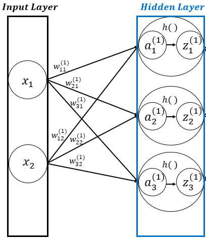
■ 이렇게 Dense Layer는 각 레이어와 레이어 사이에 모든 뉴런이 연결되어 있기 때문에 완전연결(Fully Connected) 계층이라고 부르기도 한다.
■ 따라서 완전연결 계층인 Dense Layer에 활성화 함수까지 지정한다면, Dense Layer는 '어파인 계층 + 활성화 함수 계층' 구조가 된다.
■ Dense Layer는 다음과 같이 케라스의 Layers를 이용해 구현할 수 있다.
from tensorflow.keras import layers

layers.Dense(512, input_shape=(784,))
layers.Dense(64)
layers.Dense(10)
- 입력 데이터가 784개의 열을 가지며 512개의 뉴런(노드)를 가지는 은닉층과 64개의 뉴런을 가지는 은닉층이 존재하고 출력층에는 10개의 뉴런이 있는 신경망 구조라고 생각한다면, 차원이 512 \( \rightarrow \) 64 \( \rightarrow \) 10으로 내려가는 구조라고 볼 수 있다.
■ 다만, 이렇게 활성화 함수 없이 Dense 층으로만 구성된 신경망은 아무리 깊게 Dense 층을 쌓아도 결국 하나의 선형 모델 \( y = w \cdot x + b \) 즉, 하나의 Dense 층과 같다.
- 위와 같이 연속으로 있는 2개의 Affine 층을 생각해 보자. \( affine1(x) = w_1 \cdot x + b_1 \)라고 했을 때,
- 연속으로 있는 2개의 Affine 층은 \( affine2(affine1(x)) = w_2 \cdot ( w_1 \cdot x + b_1) + b_2 = (w_2 \cdot w_1) \cdot x + (w_2 \cdot b_1 + b_2) \)이다.
- \( (w_2 \cdot w_1 = w), \quad (w_2 \cdot b_1 + b_2 = b) \)로 생각해 보면, 이는 선형 변환을 담당하는 \( w \)가 \( w_2 \cdot w_1 \)이고, 선형 변환 후 이동을 담당하는 \( + b \)가 \( w_2 \cdot b_1 + b_2 \)인 하나의 Affine 변환으로 볼 수 있다.
■ 이렇게 활성화 함수 없이 Dense 층으로만 구성된 다층 신경망은 결국 하나의 Dense 층과 같으므로, 층을 깊게 해도 선형 함수이기 때문에 비선형 문제를 해결할 수 없다. 이것이 ReLU 함수같은 비선형 함수가 필요한 이유이다.
■ 하나의 Affine 변환에 활성화 함수를 적용한 Dense 층을 중첩한 신경망 구조를 만든다면, 복잡하고 비선형적인 문제를 해결할 수 있다.
- 예를 들어, 빨간색 종이와 파란색 종이가 같이 얽혀 있을 때 빨간색 종이와 파란색 종이를 구별하는 문제는 고차원 비선형 문제이다. 비선형 함수는 원래 공간에서 구분하기 어려웠던 이 복잡한 형태를 조금씩 펼쳐서 새로운 공간에서는 두 종이를 더 쉽게 분리할 수 있도록 도와주는 역할을 한다.
■ 따라서 Dense Layer를 설정할 때 활성화 함수를 지정할 필요가 있으며, 다음과 같이 Dense Layer의 두 번째 매개변수인 activation에 활성화 함수의 이름을 명시해 주면 된다.
layers.Dense(512, input_shape=(784,))
layers.Dense(64, activation = 'relu') # 은닉층
layers.Dense(10, activation = 'softmax') # 출력층
2. Sequential API
■ 텐서플로 케라스는 3 가지 방식으로 모델을 생성할 수 있으며, 그 중 하나인 Sequential API는 주로 간단한 딥러닝 모델을 만들 때 사용한다.
■ Sequential API는 각 층을 순서에 맞춰 일렬로 연결하는 방식이다. 따라서 입력층부터 출력층까지 설정한 순서에 따라 각 층을 통과하며 딥러닝 연산이 이루어진다.
■ 순차적으로 층을 쌓아 모델을 구성하기 때문에 간단하지만, 2개 이상의 다중 입력이나 다중 출력을 갖는 복잡한 구조를 만들 수 없다는 단점이 있다. 이런 경우 Functional API를 사용해야 한다.
2.1 Sequential 모델 정의
■ Sequential API를 사용한다면 2가지 방법으로 모델을 정의할 수 있다. 가장 간단한 방법은 Sequential 클래스를 사용하는 것이다.
from tensorflow import keras
from tensorflow.keras import layers

model1 = keras.Sequential([
    layers.Dense(64, activation = 'relu'),
    layers.Dense(10, activation = 'softmax'),
], name = 'model1')
- 첫 번째 방법은 Sequential 클래스 함수에 파이썬 리스트 형태로 여러 개의 층을 넣는 것이다. 쉼표로 구분하여 층을 쌓고 앞에 위치한 층부터 순차적으로 연산을 수행한다.
■ 동일한 모델을 add( ) 메서드를 통해 층을 쌓는 형태처럼 점진적으로 만들 수도 있다.
model2 = keras.Sequential(name = 'model2')
model2.add(layers.Dense(64, activation = 'relu'))
model2.add(layers.Dense(10, activation = 'softmax'))
- 두 번째 방법은 먼저 Sequential 클래스의 객체를 만든 다음, add 함수로 객체에 레이어를 추가하는 방법이다.
- 위와 같이 하나의 add 함수를 사용해서 1개의 층을 추가할 수 있다. 따라서 여러 개의 층을 쌓으려면 그만큼 add 함수를 사용해야 한다.
■ 단, 반드시 첫 번째 층은 input_shape 매개변수를 지정하거나 입력 크기를 지정하여 build( ) 메서드를 호출해야 한다.
■ 이는 층의 가중치 크기가 입력 크기에 따라 달라지기 때문이다. 즉, 입력 크기를 설정하기 전까지 가중치를 만들 수 없다.
■ 실제로 위의 두 방법으로 만든 모델의 가중치를 확인해 보면, 다음과 같은 오류가 출력된다.
model1.weights
```#결과#```
ValueError: Weights for model model1 have not yet been created.
Weights are created when the Model is first called on inputs or `build()` is called with an `input_shape`.
````````````

model2.weights
```#결과#```
ValueError: Weights for model model2 have not yet been created.
Weights are created when the Model is first called on inputs or `build()` is called with an `input_shape`.
````````````
■ 먼저 input_shape을 사용할 경우, 다음과 같이 입력 크기를 지정할 수 있다.
- input_shape 매개변수는 입력 데이터의 shape을 튜플 혹은 리스트로 지정할 수 있다.
- 예를 들어 데이터의 shape이 (60000, 784)라면, 6만 개의 데이터에 대해 784개의 입력 변수 또는 784개의 feature가 존재한다는 뜻이다. 이때 input_shape은 (784, ) 또는 [784]로 지정할 수 있다.
### 입력 크기 input_shape으로 설정
## 1. 리스트형
model1 = keras.Sequential([
    layers.Dense(512, input_shape=(784,)),
    layers.Dense(64, activation = 'relu'),
    layers.Dense(10, activation = 'softmax')
], name = 'model1')
model1.summary()
```#결과#```
Model: "model1"
┏━━━━━━━━━━━━━━━━━━━━━━━━━━━━━━━━━━━━━━┳━━━━━━━━━━━━━━━━━━━━━━━━━━━━━┳━━━━━━━━━━━━━━━━━┓
┃ Layer (type)                         ┃ Output Shape                ┃         Param # ┃
┡━━━━━━━━━━━━━━━━━━━━━━━━━━━━━━━━━━━━━━╇━━━━━━━━━━━━━━━━━━━━━━━━━━━━━╇━━━━━━━━━━━━━━━━━┩
│ dense (Dense)                        │ (None, 512)                 │         401,920 │
├──────────────────────────────────────┼─────────────────────────────┼─────────────────┤
│ dense_1 (Dense)                      │ (None, 64)                  │          32,832 │
├──────────────────────────────────────┼─────────────────────────────┼─────────────────┤
│ dense_2 (Dense)                      │ (None, 10)                  │             650 │
└──────────────────────────────────────┴─────────────────────────────┴─────────────────┘
 Total params: 435,402 (1.66 MB)
 Trainable params: 435,402 (1.66 MB)
 Non-trainable params: 0 (0.00 B)
````````````

model1.weights
```#결과#```
[<KerasVariable shape=(784, 512), dtype=float32, path=model1/dense/kernel>,
 <KerasVariable shape=(512,), dtype=float32, path=model1/dense/bias>,
 <KerasVariable shape=(512, 64), dtype=float32, path=model1/dense_1/kernel>,
 <KerasVariable shape=(64,), dtype=float32, path=model1/dense_1/bias>,
 <KerasVariable shape=(64, 10), dtype=float32, path=model1/dense_2/kernel>,
 <KerasVariable shape=(10,), dtype=float32, path=model1/dense_2/bias>]
````````````

## 2. add 함수
model2 = keras.Sequential(name = 'model2')
model2.add(layers.Dense(512, input_shape = (784, )))
model2.add(layers.Dense(64, activation = 'relu'))
model2.add(layers.Dense(10, activation = 'softmax'))
model2.summary()
```#결과#```
Model: "model2"
┏━━━━━━━━━━━━━━━━━━━━━━━━━━━━━━━━━━━━━━┳━━━━━━━━━━━━━━━━━━━━━━━━━━━━━┳━━━━━━━━━━━━━━━━━┓
┃ Layer (type)                         ┃ Output Shape                ┃         Param # ┃
┡━━━━━━━━━━━━━━━━━━━━━━━━━━━━━━━━━━━━━━╇━━━━━━━━━━━━━━━━━━━━━━━━━━━━━╇━━━━━━━━━━━━━━━━━┩
│ dense_3 (Dense)                      │ (None, 512)                 │         401,920 │
├──────────────────────────────────────┼─────────────────────────────┼─────────────────┤
│ dense_4 (Dense)                      │ (None, 64)                  │          32,832 │
├──────────────────────────────────────┼─────────────────────────────┼─────────────────┤
│ dense_5 (Dense)                      │ (None, 10)                  │             650 │
└──────────────────────────────────────┴─────────────────────────────┴─────────────────┘
 Total params: 435,402 (1.66 MB)
 Trainable params: 435,402 (1.66 MB)
 Non-trainable params: 0 (0.00 B)
````````````

model2.weights
```#결과#```
[<KerasVariable shape=(784, 512), dtype=float32, path=model2/dense_3/kernel>,
 <KerasVariable shape=(512,), dtype=float32, path=model2/dense_3/bias>,
 <KerasVariable shape=(512, 64), dtype=float32, path=model2/dense_4/kernel>,
 <KerasVariable shape=(64,), dtype=float32, path=model2/dense_4/bias>,
 <KerasVariable shape=(64, 10), dtype=float32, path=model2/dense_5/kernel>,
 <KerasVariable shape=(10,), dtype=float32, path=model2/dense_5/bias>]
````````````
■ model.summary( )를 통해 모델 구조를 확인할 수 있다.
- 층별 뉴런(노드)의 개수와 모델 내부에 존재하는 모든 파라미터(Total params)의 개수 그리고 훈련 시 업데이트할 파라미터(Trainable params)의 개수, 훈련 시 업데이트하지 않을 파라미터(Non-trainable params)의 개수가 표기된다.
cf) 모델의 총 파라미터 수(모델 내부 가중치와 편향의 총 개수)는 435,402 개로 나왔는데,
- 이는 첫 번째 Dense 층에서 입력 데이터 수가 784개이고 두 번째 층의 뉴런이 512개이다. 그리고 Dense Layer는 use_bias = True가 기본 값이라서 자동으로 상수항 b가 추가된다.
- 따라서 첫 번째 Dense 레이어의 파라미터 수는 784 × 512에 편향 512개를 더한 401,920, 두 번째와 세번 째 층도 동일한 방식으로 계산하면 (512 × 64) + 64 = 32,832, (64 × 10) + 10 = 650. 따라서 총 파라미터 수는 401,920 + 32,282 + 650 = 435,402
- 그리고 모든 파라미터의 dtype이 float32이므로 435,402 x 4 byte = 1,741,608 byte가 된다. 1 MB = 1024 KB, 1 KB = 1024 byte이므로 1,741,608 byte를 MB 단위로 바꾸면 \(
\dfrac{1,741,608}{1,048,576} \approx 1.66 \, \text{MB}
\)가 된다.
cf) 모델의 깊이(레이어 수)와 너비(각 레이어의 뉴런 수)에 대해 정해진 정답은 없다. 최적의 모델을 찾기 위해서는 하이퍼파라미터뿐만 아니라 레이어 수와 각 층의 뉴런 수 또한 여러 번 시도하여 최적의 모델 구조를 찾아야 한다. 이러한 점에서 레이어 수와 뉴런(노드) 수 역시 중요한 하이퍼파라미터로 볼 수 있다.
■ build( ) 메서드를 사용할 경우 다음과 같다.
model1 = keras.Sequential([
    layers.Dense(512, activation = 'relu'),
    layers.Dense(64, activation = 'relu'),
    layers.Dense(10, activation = 'softmax'),
], name = 'model1')
model1.weights
```#결과#```
[]
````````````

## build( ) 메서드로 입력 크기 지정
model1.build(input_shape=(None, 784)) # 여기서 None은 어떤 배치 크기도 가능하다는 의미
model1.weights
```#결과#```
[<KerasVariable shape=(784, 512), dtype=float32, path=model1/dense_10/kernel>,
 <KerasVariable shape=(512,), dtype=float32, path=model1/dense_10/bias>,
 <KerasVariable shape=(512, 64), dtype=float32, path=model1/dense_11/kernel>,
 <KerasVariable shape=(64,), dtype=float32, path=model1/dense_11/bias>,
 <KerasVariable shape=(64, 10), dtype=float32, path=model1/dense_12/kernel>,
 <KerasVariable shape=(10,), dtype=float32, path=model1/dense_12/bias>]
````````````

model2 = keras.Sequential(name = 'model2')
model2.add(layers.Dense(512, activation = 'relu'))
model2.add(layers.Dense(64, activation = 'relu'))
model2.add(layers.Dense(10, activation = 'softmax'))
model2.weights
```#결과#```
[]
````````````

model2.build(input_shape=(None, 784))
model2.weights
```#결과#```
[<KerasVariable shape=(784, 512), dtype=float32, path=model2/dense_13/kernel>,
 <KerasVariable shape=(512,), dtype=float32, path=model2/dense_13/bias>,
 <KerasVariable shape=(512, 64), dtype=float32, path=model2/dense_14/kernel>,
 <KerasVariable shape=(64,), dtype=float32, path=model2/dense_14/bias>,
 <KerasVariable shape=(64, 10), dtype=float32, path=model2/dense_15/kernel>,
 <KerasVariable shape=(10,), dtype=float32, path=model2/dense_15/bias>]
````````````
■ 이렇게 Dense Layer로 입력 크기를 지정하거나 build( ) 메서드를 사용해서 입력 크기를 지정하지 않으면 모델 구조가 완전히 정의되지 않았으므로 가중치를 만들 수 없으며, summary( ) 메서드도 호출할 수 없다.
■ 이렇게 (1) 모델 구조를 정의하고 모델을 생성한 다음, 일반적인 딥러닝 프로세스는 다음과 같은 순서로 진행된다.
- (2) 모델 컴파일
- 모델 훈련에 사용할 손실 함수, 옵티마이저, 평가지표 등을 정의하는 단계
- (3) 모델 훈련
- 모델 훈련에 필요한 파라미터를 설정하고 모델을 훈련하는 단계. 이를 통해 손실 함수의 값이 최솟값이 될 수 있도록 가중치 매개변수를 갱신.
- (4) 모델 검증
- 훈련이 끝난 모델을 검증. 이때 사용되는 검증 데이터 셋은 모델을 훈련할 때 사용하지 않은 데이터 셋이어야 한다. 검증 결과를 토대로 모델의 잠재적인 성능을 평가한다. 평가 결과를 바탕으로 목표 성능에 도달할 때까지 다시 모델 생성 단계로 돌아가 모델을 수정, 컴파일, 훈련, 검증 과정을 반복한다.
- (5) 모델 예측
- 검증이 완료된 모델로 테스트 셋에 대해 예측하고 예측 결과를 반환한다.
2.2 Sequential 모델 컴파일
■ 컴파일 단계는 훈련 과정에 적용할 손실 함수, 옵티마이저, 평가지표 등을 정의하는 단계이다.
■ 손실 함수의 값은 훈련 과정에서 최소화할 값이며, 옵티마이저는 손실 함수를 기반으로 네트워크의 갱신과 갱신 방법을 결정한다. 측정 지표는 사용자가 지정한 손실 함수와 옵티마이저를 훈련 과정에서 모니터링할 성능 척도이다.
■ 손실 함수, 옵티마이저, 평가지표는 사용자 정의 함수로 직접 정의해서 설정하거나 클래스 인스턴스 또는 사전 정의된 문자열 사용. 이렇게 3 가지 방법으로 설정할 수 있다.
■ 클래스 인스턴스로 설정할 경우 학습률, 모멘텀 계수 등의 하이퍼파라미터를 직접 설정할 수 있지만, 문자열로 설정하는 경우 기본값으로 설정된 하이퍼파라미터가 사용되며, 하이퍼파라미터 수정이 어렵다는 단점이 있다.
# 사전 정의된 문자열로 컴파일 설정
model.compile(optimizer='adam',
              loss='categorical_crossentropy',
              metrics=['acc'])

model.compile(optimizer='adam',
              loss='categorical_crossentropy',
              metrics=['accuracy'])

# 클래스 인스턴스로 컴파일 설정
model.compile(
    optimizer = tf.keras.optimizers.Adam(learning_rate = 0.01, beta_1=0.9, beta_2=0.99),
    loss = tf.keras.losses.CategoricalCrossentropy(),
    metrics = [tf.keras.metrics.Accuracy()]

)
2.3 Sequential 모델 훈련
■ 컴파일이 완료된 모델에 fit( ) 메서드를 적용해 모델을 훈련을 통해 가중치 매개변수를 업데이트한다.
■ 가중치 매개변수를 갱신하기 위해 fit( ) 메서드에서 필요한 기본적인 정보는 훈련용 데이터 셋의 입력(x)과 입력에 따른 출력(y) 그리고 반복 훈련할 epoch 수와 각 epoch에서 사용할 배치 크기(역전파 과정에서 그래디언트를 계산하는 데 사용될 훈련 데이터의 개수)이다.
■ 만약, fit( ) 메서드에 unseen 데이터에 대한 성능을 모니터링하기 위해 검증 데이터 셋도 설정했다면, 매 epoch마다 검증 셋에 대한 손실과 평가지표도 확인할 수 있다.
# 훈련 데이터 셋만 지정
model.fit(train_set, train_labels, batch_size = 128, epochs=5)

# 검증 데이터 셋도 지정
model.fit(train_set, train_labels, batch_size = 128, validation_data=(valid_set, valid_labels), epochs=5)
■ model.fit의 결과를 history라는 변수에 대입하면 history 변수에는 epoch별 훈련 & 검증 손실과 평가지표가 딕셔너리 형태로 저장된다.
history = model.fit(train_set, train_labels, batch_size = 128, validation_data=(valid_set, valid_labels), epochs=5)
print(history.history)
```#결과#```
{'loss': [0.061744511127471924, 0.05905229225754738, 0.05555776506662369, 0.05135563760995865, 0.05956941843032837],
'categorical_accuracy': [0.9933750033378601, 0.9935208559036255, 0.9941041469573975, 0.9938958287239075, 0.9939583539962769],
'val_loss': [0.7169449329376221, 0.6773361563682556, 0.7309063076972961, 0.7119907140731812, 0.7511981725692749],
'val_categorical_accuracy': [0.9692500233650208, 0.9679166674613953, 0.9674166440963745, 0.9700000286102295, 0.9695000052452087]}
````````````
■ 이제 MNIST 데이터 셋으로 데이터 로드 \( \rightarrow \) 데이터 전처리 \( \rightarrow \) 데이터 분할 \( \rightarrow \) 모델 생성 \( \rightarrow \) 모델 컴파일 \( \rightarrow \) 훈련 \( \rightarrow \) 검증까지의 단계를 진행해 보자.
from tensorflow.keras.datasets import mnist

## 데이터 로드
(train_set, train_labels), (test_set, test_labels) = mnist.load_data()

## 데이터 전처리
train_set = train_set.reshape((60000, 28*28)) # 평탄화
train_set = train_set.astype('float32') / 255 # 정규화
test_set = test_set.reshape((10000, 28 * 28)) # 평탄화
test_set = test_set.astype('float32') / 255 # 정규화

from tensorflow.keras.utils import to_categorical

# 레이블 원핫 인코딩 # 손실 함수로 categorical_crossentropy를 사용할 것이므로
train_labels = to_categorical(train_labels)
test_labels = to_categorical(test_labels)

print(train_set.shape, test_set.shape, train_labels.shape, test_labels.shape)
```#결과#```
(60000, 784) (10000, 784) (60000, 10) (10000, 10)
````````````

## 데이터 분할
# 검증 데이터 셋 설정
from sklearn.model_selection import train_test_split

train_set, valid_set, train_labels, valid_labels = train_test_split(train_set, train_labels, test_size = 0.2, random_state = 2024)
print(train_set.shape, valid_set.shape, test_set.shape, train_labels.shape, valid_labels.shape, test_labels.shape)
```#결과#```
(48000, 784) (12000, 784) (10000, 784) (48000, 10) (12000, 10) (10000, 10)
````````````
■ 데이터를 평탄화하는 이유는 완전연결 계층의 경우 입력 데이터는 1차원이 들어가야 하기 때문이다.
■ Dense Layer는 완전연결 층이기 때문에 28 x 28 크기의 2차원 이미지를 1차원으로 평탄화해서 입력 데이터로 사용해야 한다.
- 평탄화를 적용하는 방법은 위와 같이 reshape을 이용하는 방법 외에 다음과 같이 Flatten 레이어를 사용하는 방법도 있다.
train_set.shape
```#결과#```
(60000, 28, 28)
````````````

tf.keras.layers.Flatten()(train_set).shape
```#결과#```
TensorShape([60000, 784])
````````````
■ 데이터를 정규화하는 이유는 입력 데이터가 정규화하여 모델을 학습하는 경우 경사하강법 알고리즘에 의한 수렴 속도가 비정규화된 입력 데이터로 학습했을 때보다 더 빨리 수렴하기 때문이다. 또한 local minimum에 빠지는 현상을 방지해 주는 효과도 있다.
■ 훈련 데이터의 일부를 검증 데이터로 분리해서 사용하는 이유는 검증 데이터로 모델을 훈련하지 않고 훈련에 대한 손실과 성능에 대한 측정지표를 계산하기 위해서이다.
import matplotlib.pyplot as plt
image = valid_set[11111].reshape(28, 28)
plt.imshow(image, cmap = plt.cm.binary)
plt.show()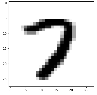
valid_labels[11111]
```#결과#```
array([0., 0., 0., 0., 0., 0., 0., 1., 0., 0.], dtype=float32)
`````````````
## 모델 생성
model = keras.Sequential([
layers.Dense(512, input_shape=(784,)),
layers.Dense(64, activation = 'relu'),
layers.Dense(10, activation = 'softmax')
])
## 모델 컴파일
model.compile(
optimizer = tf.keras.optimizers.RMSprop(learning_rate=0.001, momentum=0.5),
loss = tf.keras.losses.CategoricalCrossentropy(),
metrics = [tf.keras.metrics.CategoricalAccuracy()]
)■ 분류 모델의 손실 함수는 모델 출력층에 따라 적합한 손실 함수를 선택해야 모델이 정상적으로 훈련할 수 있다.
■ 출력층의 노드가 1개 인지, 2개 이상인지 그리고 레이블에 원핫 인코딩을 적용했는지에 따라 선택해야 할 손실 함수가 달라진다.
- 마지막 출력층의 노드 개수가 1개면, 출력층의 활성화 함수는 sigmoid, 손실 함수는 binary_crossentropy
- 마지막 출력층의 노드 개수가 2개 이상이면, 출력층의 활성화 함수는 softmax를 사용한다. 이때 레이블이 원핫 벡터인 경우 categorical_crossentropy를, 원핫 벡터가 아닌 경우 sparse_categorical_crossentropy를 사용한다.
## 모델 훈련 및 검증
history = model.fit(train_set, train_labels, batch_size = 512, validation_data=(valid_set, valid_labels), epochs=100)
```#결과#```
Epoch 1/100
94/94 ━━━━━━━━━━━━━━━━━━━━ 1s 8ms/step - categorical_accuracy: 0.7823 - loss: 0.6614 - val_categorical_accuracy: 0.9369 - val_loss: 0.2184
...,
...,
Epoch 100/100
94/94 ━━━━━━━━━━━━━━━━━━━━ 1s 6ms/step - categorical_accuracy: 0.9975 - loss: 0.0100 - val_categorical_accuracy: 0.9730 - val_loss: 0.3337
````````````

## 결과 시각화
# 손실 값 변화 그래프
import matplotlib.pyplot as plt

plt.plot(history.history['loss'], label='Training Loss')
plt.plot(history.history['val_loss'], label='Validation Loss')
plt.xlabel('Epochs')
plt.ylabel('Loss')
plt.legend()
plt.show()

# 정확도 변화 그래프
plt.plot(history.history['categorical_accuracy'], label='Training Accuracy')
plt.plot(history.history['val_categorical_accuracy'], label='Validation Accuracy')
plt.xlabel('Epochs')
plt.ylabel('Accuracy')
plt.legend()
plt.show()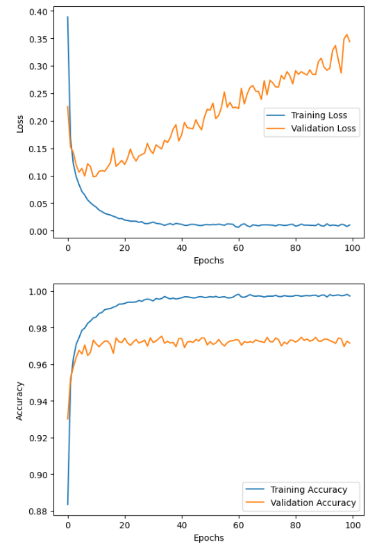
■ 결과를 봤을 때, 먼저 눈에 보이는 것은 훈련 데이터에 잘 작동하지만 처음 보는 검증 데이터에선 잘 작동하지 않는 즉, 과대적합(overfitting)이 발생한다는 점이다. 오버피팅은 loss가 급격히 감소하는 10 epoch 부근부터 발생한 것으로 보인다. valid loss의 값도 점차 커지는 것을 볼 수 있다.
■ train loss가 급격히 감소하다가 감소 폭이 둔화되는 것을 볼 수 있는데, 이는 학습 초기에 학습이 매우 빠른 속도로 진행되다가 일정 epcoh 이후에는 학습 속도가 느려진 것이다. 즉, 10 epoch 이후 훈련용 데이터 셋은 손실 함수의 최솟값에 도달해 가는 것으로 볼 수 있으며, 반대로 valid loss는 손실 함수의 값이 점차 커지는 것으로 보아 최솟값을 찾지 못하는 것으로 볼 수 있다.
■ 과대적합을 확인한 후, 확인해야 할 다른 포인트는 바로 과소적합이다. 훈련 초기 10 epoch 이전 훈련 데이터의 손실이 낮아질수록 검증 데이터의 손실도 낮아지는 것을 볼 수 있다. 이런 상황이 발생했을 때 모델이 과소적합되었다고 말한다.
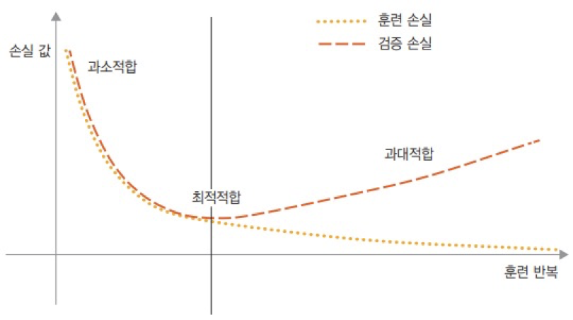
■ 이렇게 과소적합과 과대적합을 확인해야 하는 이유는 모델 성능이 개선될 여지가 있는지, 즉 최적적합이 되는 지점을 찾기 위해서이다. 최적적합 지점은 다음 그림과 같이 과소적합과 과대적합 사이에 존재하기 때문이다.
2.4 Sequential 모델 검증
■ 모델 훈련이 끝나면(fit( ) 메서드에 validation set을 지정해서 훈련한 경우) evaluate( ) 메소드에 테스트 데이터 셋을 넣어 unseen 데이터에 대한 모델의 성능을 확인할 수 있다.
model.evaluate(test_set, test_labels)
```#결과#```
313/313 ━━━━━━━━━━━━━━━━━━━━ 0s 844us/step - categorical_accuracy: 0.9687 - loss: 0.3976
[0.3306841552257538, 0.9729999899864197]
````````````
2.5 Sequential 모델 예측
■ 모델 훈련과 검증이 끝나면 predict( ) 메소드에 새로운 입력 데이터를 넣어 모델의 예측 값을 구할 수 있다.
pred = model.predict(test_set)
pred[0]
```#결과#```
array([0.0000000e+00, 7.1943147e-35, 4.5373804e-27, 1.5985991e-15,
       0.0000000e+00, 0.0000000e+00, 0.0000000e+00, 1.0000000e+00,
       5.0291327e-27, 9.4004289e-26], dtype=float32)
````````````
- 출력층 함수로 softmax 함수를 사용했기 때문에 10개의 출력 클래스에 대한 확률 분포를 출력한다.
- 따라서 pred[0]은 10가지 클래스 중에 7번째 클래스일 확률이 가장 크다는 것 의미한다. 실제 정답도 7 번째 클래스임을 볼 수 있다.
## 예측한 클래스
np.argmax(pred[0])
```#결과#```
7
````````````

## 실제 정답
test_labels[0]
```#결과#```
array([0., 0., 0., 0., 0., 0., 0., 1., 0., 0.])
````````````
3. 모델 세부 설정
3.1 가중치 초깃값 설정
■ Dense 레이어는 가중치 초기화 기본값이 S자 곡선 형태의 함수에 적합한 Glorot Uniform, Xavier의 균등 분포 초기화로 설정되어 있다.
dense = layers.Dense(100, activation = 'sigmoid')
dense.get_config()['kernel_initializer']
```#결과#```
{'class_name': 'GlorotUniform', 'config': {'seed': None}}
````````````
■ 모델 훈련 과정에서 순전파와 역전파가 진행되는 만큼 각 층의 활성화 함수에 적합한 가중치 초깃값을 설정해야 한다.
매개변수 갱신 방법(2) - 가중치 초깃값, 규제, 드롭아웃, 배치 정규화
매개변수 갱신 방법(2)
1. 가중치 초깃값■ 너무 큰 가중치 (매개변수)값은 학습 과정에서 과적합을 발생시킬 수 있어서 초깃값을 최대한 작은 값에서 시작하거나 가중치 감소 기법을 통해 과적합을 억제해야 한다.■
hyeon-jae.tistory.com
■ 케라스에서 지원하는 가중치 초깃값 목록은 다음과 같다.
Module: tf.keras.initializers | TensorFlow v2.16.1
Module: tf.keras.initializers | TensorFlow v2.16.1
DO NOT EDIT.
www.tensorflow.org
■ 위의 MNIST 모델에서는 은닉층의 활성화 함수로 비선형 함수인 ReLU 함수를 사용했다. 따라서 가중치 초깃값을 He 초깃값으로 변경해주는 것이 좋다.
- 케라스는 He 초깃값의 정규 분포 방법(HeNormal)과 균등 분포 방법(HeUniform)을 모두 지원한다.
■ 가중치 초깃값을 지정하는 방법은 다음과 같이 kernel_initializer 매개변수에 클래스 인스턴스로 지정하는 방법과 문자열로 지정하는 방법이 있다.
# 클래스 인스턴스로 설정
initializer = tf.keras.initializers.HeNormal(seed=None)
dense2 = layers.Dense(100, kernel_initializer = initializer, activation = 'relu')
print(dense2.get_config()['kernel_initializer'])
```#결과#```
{'class_name': 'HeNormal', 'config': {'seed': None}}
````````````

# 문자열로 설정
dense3 = layers.Dense(100, kernel_initializer = 'HeUniform', activation = 'relu')
print(dense3.get_config()['kernel_initializer'])
```#결과#```
{'class_name': 'HeUniform', 'config': {'seed': None}}
````````````
3.2 규제(Regularization)
■ 과대적합을 완화하기 위해 모델의 복잡도에 제한을 두어 가중치가 작은 값을 가지도록 강제하는 방법이 규제이다. 가중치 규제에 따라 가중치 값의 분포가 더 균일하게 된다. 이를 가중치 규제라고 하며, 모델의 손실 함수에 큰 가중치에는 큰 페널티, 작은 가중치에는 작은 페널티를 부과한다.
■ 규제 방법으로 L1, L2 규제가 있다. L1 규제는 가중치의 절댓값에 비례하는 비용, L2는 가중치의 제곱에 비례하는 비용을 추가한다. L2 규제는 신경망에서 가중치 감쇠(weight decay)라고도 부른다.
■ 케라스에서 모델의 오버피팅을 억제하기 위해 페널티를 부과하는 L1, L2 규제를 설정할 수 있다. 단, 텐서플로 케라스 레이어에서는 기본값으로 규제를 적용하고 있지 않다.
dense.get_config()
```#결과#```
{'name': 'dense_5',
 'trainable': True,
 'dtype': 'float32',
 'units': 100,
 'activation': 'sigmoid',
 'use_bias': True,
 'kernel_initializer': {'class_name': 'GlorotUniform',
  'config': {'seed': None}},
 'bias_initializer': {'class_name': 'Zeros', 'config': {}},
 'kernel_regularizer': None,
 'bias_regularizer': None,
 'activity_regularizer': None,
 'kernel_constraint': None, ## 규제 기본값
 'bias_constraint': None}
````````````
■ 따라서 Dense 레이어의 kernel_regularizer 매개변수에 사용할 규제 방법을 별도로 지정해야 한다.
Module: tf.keras.regularizers | TensorFlow v2.16.1
Module: tf.keras.regularizers | TensorFlow v2.16.1
DO NOT EDIT.
www.tensorflow.org
■ 케라스에서는 Dense Layer에 'kernel_regularizer' 매개변수에 문자열을 지정하여 가중치 규제를 추가할 수 있고, regularizers.l1( ), regularizers.l2( ) , regularizers.l1l2( ) 함수를 지정해 가중치 규제를 추가할 수도 있다.
cf) regularizers.l1l2( )는 L1과 L2 규제를 함께 쓰는 방식이며, 이를 엘라스틱넷(ElasticNet)이라고도 부른다.
■ 규제도 클래스 인스턴스, 문자열로 다음과 같이 지정할 수 있으며 L1, L2, L1L2 함수의 기본값은 모두 0.01이다.
# L1 규제 설정
## 문자열로 설정
dense2 = layers.Dense(100, kernel_initializer = initializer, kernel_regularizer = 'l1', activation = 'relu') # defalut 값 L1 = 0.01
print(dense2.get_config()['kernel_regularizer'])
```#결과#```
{'class_name': 'L1', 'config': {'l1': 0.009999999776482582}}
````````````

# L2 규제 설정
## 클래스 인스턴스로 설정
regularizer = tf.keras.regularizers.L2(l2 = 0.01)
dense3 = layers.Dense(100, kernel_initializer = 'HeUniform', kernel_regularizer = regularizer, activation = 'relu')
print(dense3.get_config()['kernel_regularizer'])
```#결과#```
{'class_name': 'L2', 'config': {'l2': 0.009999999776482582}}
````````````
■ 가중치 규제는 보통 작은 용량의 딥러닝 모델에서 사용된다. 왜냐하면, 대규모 용량의 딥러닝 모델은 파라미터가 너무 많아서 가중치 값에 제약(페널티 부과)을 걸어도 모델 용량과 성능 일반화에 큰 영향을 미치지 않는 경향이 있기 때문이다.
3.3 드롭아웃(Dropout)
■ 위에서 언급한 것처럼 대규모 용량의 딥러닝 모델은 파라미터가 너무 많기 때문에 파라미터에 가중치 제약을 걸어도 영향이 미미하다.
■ 따라서 아예 각 샘플에 대해 뉴런의 일부를 무작위로 '제거'하는 방법으로 파라미터를 억제하여 과대적합을 감소시키는 방법이 바로 드롭아웃이다.
■ 케라스에서는 Dropout 층을 추가하고 드롭아웃 비율을 설정하는 방법으로 드롭아웃을 구현할 수 있다.
tf.keras.layers.Dropout | TensorFlow v2.16.1
tf.keras.layers.Dropout | TensorFlow v2.16.1
Applies dropout to the input.
www.tensorflow.org
tf.keras.layers.Dropout(rate = 0.5, noise_shape=None, seed=None)
3.4 배치 정규화(Batch Normalization)
■ 케라스는 배치 정규화 레이어를 지원한다.
tf.keras.layers.BatchNormalization | TensorFlow v2.16.1
tf.keras.layers.BatchNormalization | TensorFlow v2.16.1
Layer that normalizes its inputs.
www.tensorflow.org
tf.keras.layers.BatchNormalization()■ 배치 정규화의 목적은 각 층에서 활성화 값들이 적절한 분포를 갖게 하여 역전파 과정에서도 적절한 기울기가 유지되도록 하는 것이다. 이를 위해 배치 정규화 계층을 활성화 함수 계층의 앞 혹은 뒤에 위치시켜 각 층에서 데이터 분포를 덜 치우치게 만들어 준다.
■ 배치 정규화 계층을 삽입한 모델과 그렇지 않은 모델의 성능을 비교해보면
initializer = tf.keras.initializers.HeNormal(seed=2024)

model_A = tf.keras.Sequential([
    tf.keras.layers.Flatten(input_shape = (28, 28)),
    tf.keras.layers.Dense(256, kernel_initializer = initializer, activation = 'relu'),
    tf.keras.layers.Dense(64, kernel_initializer = initializer, activation = 'relu'),
    tf.keras.layers.Dense(32, kernel_initializer = initializer, activation = 'relu'),
    tf.keras.layers.Dense(16),
    tf.keras.layers.Dense(10, activation = 'softmax')
])

model_A.summary()
```#결과#```
Model: "sequential_25"
_________________________________________________________________
 Layer (type)                Output Shape              Param #
=================================================================
 flatten_19 (Flatten)        (None, 784)               0

 dense_83 (Dense)            (None, 256)               200960

 dense_84 (Dense)            (None, 64)                16448

 dense_85 (Dense)            (None, 32)                2080

 dense_86 (Dense)            (None, 16)                528

 dense_87 (Dense)            (None, 10)                170

=================================================================
Total params: 220,186
Trainable params: 220,186
Non-trainable params: 0
_________________________________________________________________
````````````

model_B = tf.keras.Sequential([
    tf.keras.layers.Flatten(input_shape = (28, 28)),

    # Affine + Activation Function + Batch Norm  # 활성화 함수 계층 뒤에 배치 정규화 계층을 배치
    tf.keras.layers.Dense(256, kernel_initializer = initializer, activation = 'relu'),
    tf.keras.layers.BatchNormalization(),

    tf.keras.layers.Dense(64, kernel_initializer = initializer, activation = 'relu'),
    tf.keras.layers.BatchNormalization(),

    tf.keras.layers.Dense(32, kernel_initializer = initializer, activation = 'relu'),
    tf.keras.layers.BatchNormalization(),

    tf.keras.layers.Dense(16),
    tf.keras.layers.Dense(10, activation = 'softmax')
])

model_B.summary()
```#결과#```
Model: "sequential_26"
_________________________________________________________________
 Layer (type)                Output Shape              Param #
=================================================================
 flatten_20 (Flatten)        (None, 784)               0

 dense_88 (Dense)            (None, 256)               200960

 batch_normalization_31 (Bat  (None, 256)              1024
 chNormalization)

 dense_89 (Dense)            (None, 64)                16448

 batch_normalization_32 (Bat  (None, 64)               256
 chNormalization)

 dense_90 (Dense)            (None, 32)                2080

 batch_normalization_33 (Bat  (None, 32)               128
 chNormalization)

 dense_91 (Dense)            (None, 16)                528

 dense_92 (Dense)            (None, 10)                170

=================================================================
Total params: 221,594
Trainable params: 220,890
Non-trainable params: 704
````````````
model_A.compile(
optimizer = tf.keras.optimizers.RMSprop(learning_rate=0.001, momentum=0.5),
loss = tf.keras.losses.CategoricalCrossentropy(),
metrics = [tf.keras.metrics.CategoricalAccuracy()]
)
model_B.compile(
optimizer = tf.keras.optimizers.RMSprop(learning_rate=0.001, momentum=0.5),
loss = tf.keras.losses.CategoricalCrossentropy(),
metrics = [tf.keras.metrics.CategoricalAccuracy()]
)
from tensorflow.keras.datasets import mnist
(train_set, train_labels), (test_set, test_labels) = mnist.load_data()
train_set = train_set.astype('float32') / 255 # 정규화
test_set = test_set.astype('float32') / 255 # 정규화
train_labels = to_categorical(train_labels) # 원핫 인코딩
test_labels = to_categorical(test_labels) # 원핫 인코딩
train_set, valid_set, train_labels, valid_labels = train_test_split(train_set, train_labels, test_size = 0.2, random_state = 2024)history_A = model_A.fit(train_set, train_labels, batch_size = 256, validation_data=(valid_set, valid_labels), epochs=100)
history_B = model_B.fit(train_set, train_labels, batch_size = 256, validation_data=(valid_set, valid_labels), epochs=100)
plt.plot(np.arange(1, 101), history_A.history['val_loss'])
plt.plot(np.arange(1, 101), history_B.history['val_loss'])
plt.legend(['Affine + ReLU', 'Affine + ReLU + Batch Norm'])
plt.show()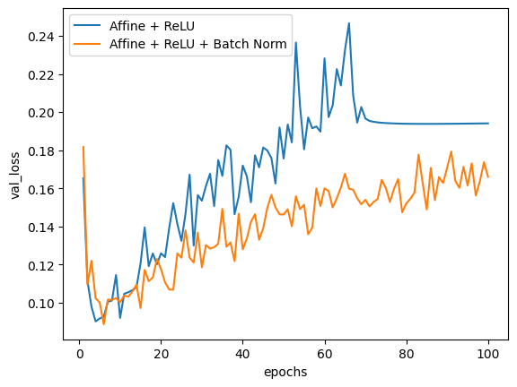
초기, 두 방법 모두 loss 값에 큰 차이가 없고 epoch 횟수가 증가할수록 loss 값이 커지지만, 배치 정규화를 추가한 모델이 그렇지 않은 모델에 비해 loss 값이 더 안정적인 것을 볼 수 있다.
3.5 활성화 함수
■ 지금까지는 주로 활성화 함수 ReLU를 Dense 레이어에 지정하여 사용하였는데, 이 방법 말고 활성화 함수를 설정할 때 클래스 인스턴스로 선언해 하이퍼파라미터 값을 변경해서 설정할 수 있다.
tf.keras.layers.LeakyReLU(alpha = 0.3)Module: tf.keras.activations | TensorFlow v2.16.1
Module: tf.keras.activations | TensorFlow v2.16.1
DO NOT EDIT.
www.tensorflow.org
Module: tf.keras.layers | TensorFlow v2.16.1
Module: tf.keras.layers | TensorFlow v2.16.1
DO NOT EDIT.
www.tensorflow.org
■ 이번에는 LeakyReLU 활성화 함수를 사용하고 Affine + Batch Norm + Activation으로 활성화 함수 앞에 배치 정규화 층을 배치해서 앞의 두 방법과 비교해 보자.
model_C = tf.keras.Sequential([
    tf.keras.layers.Flatten(input_shape = (28, 28)),

    # Affine + Batch Norm + Activation Function  # 활성화 함수 계층 앞에 배치 정규화 계층을 배치
    tf.keras.layers.Dense(256), # Affine
    tf.keras.layers.BatchNormalization(), # Batch
    tf.keras.layers.LeakyReLU(alpha = 0.3), # Activation

    tf.keras.layers.Dense(64),
    tf.keras.layers.BatchNormalization(),
    tf.keras.layers.LeakyReLU(alpha = 0.3),

    tf.keras.layers.Dense(32),
    tf.keras.layers.BatchNormalization(),
    tf.keras.layers.LeakyReLU(alpha = 0.3),

    tf.keras.layers.Dense(16),
    tf.keras.layers.Dense(10, activation = 'softmax')
])

model_C.summary()
```#결과#```
Model: "sequential_27"
_________________________________________________________________
 Layer (type)                Output Shape              Param #
=================================================================
 flatten_21 (Flatten)        (None, 784)               0

 dense_93 (Dense)            (None, 256)               200960

 batch_normalization_34 (Bat  (None, 256)              1024
 chNormalization)

 leaky_re_lu_2 (LeakyReLU)   (None, 256)               0

 dense_94 (Dense)            (None, 64)                16448

 batch_normalization_35 (Bat  (None, 64)               256
 chNormalization)

 leaky_re_lu_3 (LeakyReLU)   (None, 64)                0

 dense_95 (Dense)            (None, 32)                2080

 batch_normalization_36 (Bat  (None, 32)               128
 chNormalization)

 leaky_re_lu_4 (LeakyReLU)   (None, 32)                0

 dense_96 (Dense)            (None, 16)                528

 dense_97 (Dense)            (None, 10)                170

=================================================================
Total params: 221,594
Trainable params: 220,890
Non-trainable params: 704
_________________________________________________________________
````````````
model_C.compile(
optimizer = tf.keras.optimizers.RMSprop(learning_rate=0.001, momentum=0.5),
loss = tf.keras.losses.CategoricalCrossentropy(),
metrics = [tf.keras.metrics.CategoricalAccuracy()]
)
history_C = model_C.fit(train_set, train_labels, batch_size = 256, validation_data=(valid_set, valid_labels), epochs=100)plt.plot(np.arange(1, 101), history_A.history['val_loss'])
plt.plot(np.arange(1, 101), history_B.history['val_loss'])
plt.plot(np.arange(1, 101), history_C.history['val_loss'])
plt.legend(['Affine + ReLU', 'Affine + ReLU + Batch Norm', 'Affine + Batch Norm + LeakyReLU'])
plt.xlabel('epochs')
plt.ylabel('val_loss')
plt.show()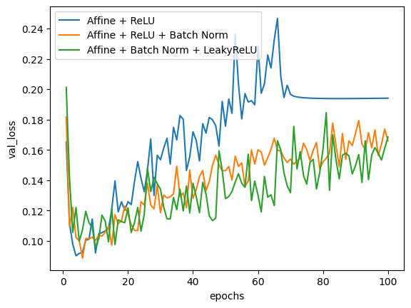
실행 결과를 보면, 배치 정규화 적용 유무가 데이터의 개수가 10만 개 미만인 MNIST 모델 성능에도 영향을 미치는 것을 볼 수 있다. MNIST set보다 더 크고 복잡한 data set에서는 모델 성능에 크게 영향을 미칠 수도 있다.
'텐서플로' 카테고리의 다른 글
| 임베딩(Embedding) 순환신경망(Recurrent Neural Network, RNN) (0) | 2025.01.21 |
|---|---|
| 텐서플로 합성곱 신경망(CNN) (2) (0) | 2024.11.22 |
| 텐서플로 합성곱 신경망(CNN) (1) (0) | 2024.11.15 |
| 케라스(Keras) (2) (2) | 2024.08.20 |
| 텐서(Tensor) (1) (0) | 2024.08.10 |


