4. 데이터 증강(Data Augmentation)
■ CNN을 포함한 딥러닝 모델은 이미지 특징을 학습하는 것이 주목적이며, 복잡한 문제를 해결하기 위해 층(layer)이 깊어진다.
■ 어느 정도 층이 깊어지면 표현력이 향상되고 일반화 성능도 보장되는데, 층이 깊어질수록 신경망 모델은 수십, 수백만 개의 파라미터를 갖게 된다.
■ 수많은 파라미터를 가진 심층 신경망 모델이 좋은 성능을 발휘하기 위해서는 그만큼 많은 데이터를 이용한 훈련이 필요하며, 이를 위한 방법으로 데이터 증강이 활용된다.
■ 현실 세계 (이미지) 데이터는 보는 각도와 밝기에 따라 전혀 다른 픽셀 값들을 가지고 있으며, 온전한 형태가 아닌 겹치거나 가려져 있을 수 있는데, 데이터 증강으로 이런 현실 세계를 모두 담을 수 없는 데이터 세트의 한계를 극복하고 정확도를 높일 수 있다.
■ 데이터 증강은 학습 이미지 데이터들을 이미지 프로세싱 알고리즘을 통해 인위적으로 이미지 데이터를 변형하는 것으로, 대표적인 방법에는 뒤집기(flip), 회전(rotation), 자르기(crop), 크기 변환(scale) 등이 있다.
■ 이렇게 데이터 증강을 적용하면 변형된 데이터로 데이터 개수를 늘리고, 같은 이미지라도 픽셀 값이 달라지므로 컨볼루션 연산을 통해 다양한 피처를 학습(추출) 할 수 있게 된다.
■ torchvision 패키지를 이용해 데이터 증강을 수행할 수 있다.
import cv2

def show_image(image):
    rgb = cv2.cvtColor(image, cv2.COLOR_BGR2RGB)
    plt.figure()
    plt.imshow(rgb)
    plt.show()

img = cv2.imread('cat1.jpg')
img.shape
```#결과#```
(145, 216, 3)
````````````
show_image(img)
- 예시 이미지는 145 x 216 크기의 컬러 이미지임을 확인할 수 있다.
class TorchvisionDataset(Dataset): # transform 패키지로 이미지를 열어 변형
    def __init__(self, file_paths, labels, transform=None):
        self.file_paths = file_paths # 이미지 파일 경로의 리스트
        self.labels = labels # 이미지 레이블의 리스트
        self.transform = transform # 이미지에 적용할 전처리 함수

    def __len__(self):
        return len(self.file_paths) # 데이터셋의 전체 샘플 개수 반환

    def __getitem__(self, idx): # idx는 샘플의 인덱스
        label = self.labels[idx]
        file_path = self.file_paths[idx]
        # 이미지 읽기
        image = Image.open(file_path)
        # 이미지 변경 수행
        if self.transform: # 이미지에 전처리 함수(Resize, RandomCrop, RandomHorizontalFlip, ToTensor 등)
            image = self.transform(image) # 를 적용
        return image, label
torchvision_transform = transforms.Compose([
transforms.Resize((220, 220)), # 이미지 크기를 220 x 220으로 조정
transforms.RandomCrop(100), # 크기 100으로 무작위 자르기
transforms.RandomHorizontalFlip(), # 이미지를 50% 확률로 좌우 반전
transforms.ToTensor(), # 0에서 1 사이의 값으로 정규화
])
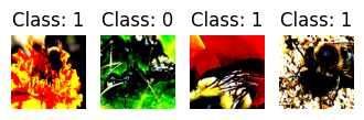
torchvision_cat_img = TorchvisionDataset(
file_paths=['cat1.jpg'],
labels=[1],
transform=torchvision_transform,
)
fig, axes = plt.subplots(2, 2)
axes = axes.ravel()
for i in range(4):
sample, _ = torchvision_cat_img[0]
axes[i].imshow(transforms.ToPILImage()(sample))
axes[i].axis('off')
plt.tight_layout()
plt.show()■ albumentations 패키지를 이용해서도 이미지 크기 변경, 랜덤 자르기, 회전, 뒤집기, 가우시안 노이즈 등의 데이터 증강을 수행할 수 있다.
■ 앞서 언급한 flip, rotation, crop 등은 데이터 증강 기법은 기본적으로 많이 사용하는 기법이고 비교적 최근에 제안된 기법으로 Cutout과 Cutmix가 있다.
- Cutout은 이미지 일부를 검은색 사각형으로 가리는 기법이다. 이미지 일부를 검은색(픽셀 값 0)으로 마스킹하는 이 방식은 이미지 데이터에 대한 드롭아웃을 적용한 기법으로 볼 수 있다.
- 그러나 Cutout은 이미지 일부분의 픽셀 값이 0이 되기 때문에 이미지 일부분을 아예 삭제한 것이며, 이는 정보 손실을 유발한다. 이런 Cutout의 문제점을 개선한 기법이 바로 Cutmix이다.
- Cutmix는 이미지 일부분을 다른 이미지의 패치로 채우는 기법으로, 두 이미지를 합쳐 놓고 이미지의 레이블을 학습시킬 때 각각의 이미지가 차지하는 비율만큼 학습시키는 방법이다.
■ 파이토치에서 다음과 같이 데이터를 불러올 때 torchvision의 transforms 함수를 이용해 데이터 증강을 적용할 수 있다. 일반적으로 학습 데이터에 이용하는 전처리 과정은 검증 데이터에도 동일하게 적용한다. 그래야 모델의 성능을 평가할 수 있기 때문이다.
train_dataset = datasets.CIFAR10(root = "../data/CIFAR_10",
                                  train = True,
                                  download = True,
                                  transform = transforms.Compose([
                                      transforms.CenterCrop(28),
                                     # transforms.RandomRotation(90),
                                      transforms.RandomHorizontalFlip(p = 0.5),
                                     # transforms.GaussianBlur(kernel_size = 3),
                                      transforms.ToTensor(),
                                      transforms.Normalize(mean = [0.5, 0.5, 0.5],
                                                           std = [0.5, 0.5, 0.5])
                                  ]))

test_dataset = datasets.CIFAR10(root = "../data/CIFAR_10",
                                train = False,
                                  transform = transforms.Compose([
                                      transforms.CenterCrop(28),
                                     # transforms.RandomRotation(90),
                                      transforms.RandomHorizontalFlip(p = 0.5),
                                     # transforms.GaussianBlur(kernel_size = 3),
                                      transforms.ToTensor(),
                                      transforms.Normalize(mean = [0.5, 0.5, 0.5],
                                                           std = [0.5, 0.5, 0.5])
                                  ]))
- transforms.Compose( )는 불러오는 이미지 데이터에 전처리 및 증강을 적용할 때 사용하는 메서드이다. 위와 같이 transforms에 여러 단계가 있는 경우, Compose를 통해 여러 단계를 하나로 묶어 한번에 처리할 수 있다.
- CenterCrop( )은 무작위로 텐서 이미지를 자르는 RandomCrop( )과 달리, 중앙에서 주어진 텐서 이미지를 자른다.
- RandomRotation( )은 이미지를 지정한 각도만큼 무작위로 회전한다.
- RandomHorizontalFlip( )은 무작위로 이미지 수평 뒤집기, RandomVerticalFlip( )는 무작위로 이미지 수직 뒤집기를 수행한다. 이미지가 뒤집힐 확률 p를 지정할 수 있으며 기본값은 0.5이다.
- GaussianBlur( )는 가우시안 분포 공식을 이용해서 이미지를 흐리게 처리하는 기법으로, 이미지에 적용할 필터(커널)의 크기를 kernel_size에 지정해서 흐림 처리 정도를 조정할 수 있다. 필터의 크기가 클수록 흐림 처리 정도가 커진다.
- 또한, sigma( )를 통해 이미지 x, y축 방향에 각각 얼마의 표준편차를 적용할 것인지 설정할 수 있다.
https://pytorch.org/vision/main/generated/torchvision.transforms.GaussianBlur.html
GaussianBlur — Torchvision main documentation
Shortcuts
pytorch.org
- ToTensor( )는 PIL Image나 넘파이를 FloatTensor로 변환하고, 모델의 Input으로 들어갈 수 있도록 이미지의 픽셀 값을 0에서 1 사이의 값으로 정규화를 수행한다.
- Normalize( )는 ToTensor( ) 형태로 전환된 텐서 (이미지)를 가져와 평균 및 표준편차로 또 다른 정규화를 수행한다. 그러므로 ToTensor를 사용할 경우 Normalize 전에 ToTensor를 수행해야 한다.
- 이 예의 이미지는 컬러 이미지이므로 3개의 채널 red, green, blue 채널로 이뤄져 있다.
- 이 예에서는 red, green, blue 순으로 평균을 0.5씩 적용하고 표준편차를 0.5씩 적용하였다.
5. 전이 학습(Transfer Learning)
■ 보유하고 있는 이미지의 수가 적다면 일반적인 방법으로는 이미지의 feature를 충분히 학습(추출)하기 어렵기 때문에 모델 성능에 대해 일반화를 기대하기는 어렵다.
■ 이번에 사용할 개미 vs 벌 데이터 셋은 개미와 벌 각각 학습용 이미지는 대략 120장이고, 검증용 이미지는 75개이다. 이렇게 데이터 수가 적은 경우 데이터 증강과 전이 학습을 이용하면 더 개선된 성능을 기대할 수 있다.
https://tutorials.pytorch.kr/beginner/transfer_learning_tutorial.html
컴퓨터 비전(Vision)을 위한 전이학습(Transfer Learning)
Author: Sasank Chilamkurthy, 번역: 박정환,. 이 튜토리얼에서는 전이학습(Transfer Learning)을 이용하여 이미지 분류를 위한 합성곱 신경망을 어떻게 학습시키는지 배워보겠습니다. 전이학습에 대해서는 CS
tutorials.pytorch.kr
import os
data_transforms = {
    'train': transforms.Compose([
        transforms.RandomResizedCrop(224),
        transforms.RandomHorizontalFlip(),
        transforms.ToTensor(),
        transforms.Normalize([0.485, 0.456, 0.406], [0.229, 0.224, 0.225])
    ]),
    'val': transforms.Compose([
        transforms.Resize(256),
        transforms.CenterCrop(224),
        transforms.ToTensor(),
        transforms.Normalize([0.485, 0.456, 0.406], [0.229, 0.224, 0.225])
    ]),
}

data_dir = 'data/hymenoptera_data'
image_datasets = {x: datasets.ImageFolder(os.path.join(data_dir, x),
                                          data_transforms[x])
                  for x in ['train', 'val']}
dataloaders = {x: torch.utils.data.DataLoader(image_datasets[x], batch_size=4,
                                             shuffle=True, num_workers=0)
              for x in ['train', 'val']}
dataset_sizes = {x: len(image_datasets[x]) for x in ['train', 'val']}
class_names = image_datasets['train'].classes
- train 폴더와 val 폴더에 접근해서 이미지 데이터를 불러온 다음, 이미지를 미니배치 단위로 구분하기 위해 DataLoader 함수를 사용한다.
- 여기서 num_workers는 멀티 프로세싱으로 기본값은 0이다. 프로세스를 동시에 처리하는 개수만큼 num_workers에 값을 지정한다.
- dataloaders에는 학습 데이터셋과 검증 데이터셋이 딕셔너리로 저장되는데 shuffle = True로 설정하면 데이터의 순서를 섞는다.
for (X_train, y_train) in dataloaders['train']:
    print('X_train:', X_train.size(), 'type:', X_train.type())
    print('y_train:', y_train.size(), 'type:', y_train.type())
    break

```#결과#```
X_train: torch.Size([4, 3, 224, 224]) type: torch.FloatTensor
y_train: torch.Size([4]) type: torch.LongTensor
````````````
- 이미지는 224 x 224크기의 컬러 이미지임을 확인할 수 있다.
■ 이런 상황에서는 (ImageNet 데이터를 학습한) 사전 학습(pre-trained) 모델을 불러와서 파인튜닝(fine-tuning)하는 방법을 사용하며, 이를 전이 학습이라고 한다.
■ 이때, 분류하고자 하는 문제가 다른 경우 일반적으로 완전연결 계층을 새롭게 정의해서 사전 학습 모델의 기존 완전연결 계층을 대체한다.
■ 파이토치는 torchvision.models에서 사전 훈련(pre-trained) 모델 로드가 가능하다.
https://pytorch.org/vision/0.9/models.html
torchvision.models — Torchvision master documentation
torchvision.models The models subpackage contains definitions of models for addressing different tasks, including: image classification, pixelwise semantic segmentation, object detection, instance segmentation, person keypoint detection and video classific
pytorch.org
■ 모델 구조와 함께 ImageNet 데이터에 미리 학습된 파라미터도 같이 불러오고 싶으면 pretrained = True로 설정하면 된다.
■ pretrained = False로 설정하면 모델의 구조만 불러오고 모델 구조 내에 존재하는 파라미터를 특정 초깃값에서 랜덤으로 샘플링한 값을 사용한다.
■ 미리 학습된 파라미터를 사용하는 것이 아예 랜덤으로 설정된 파라미터 값을 이용하는 것보다는 도움이 될 수 있다.
■ 분류하고자 하는 이미지 데이터와 아주 비슷한 이미지 데이터에서 학습된 모델을 이용할 수 있다면, 분류하려는 이미지 데이터에도 잘 작동할 가능성이 매우 높을 수밖에 없다.
■ 예를 들어 늑대와 호랑이 사진을 분류하는 문제에서 비행기와 배 사진을 잘 분류하는 모델을 이용하는 것보다 고양이와 강아지 사진을 잘 분류하는 모델을 이용하는 것이 바람직하다.
■ 파이토치에서 미리 학습된 파라미터를 불러오는 방법은 다음과 같이 pretrained에 True를 지정할 수도 있고 weights에 사용할 파라미터를 지정해서 불러올 수도 있다.
import torchvision.models as models
from torchsummary import summary

model = models.resnet18(pretrained = True)
model.to(DEVICE) # 또는 model = model.cuda()

summary(model, input_size = (3, 224, 224))
```#결과#```
----------------------------------------------------------------
        Layer (type)               Output Shape         Param #
================================================================
            Conv2d-1         [-1, 64, 112, 112]           9,408
       BatchNorm2d-2         [-1, 64, 112, 112]             128
              ReLU-3         [-1, 64, 112, 112]               0
         MaxPool2d-4           [-1, 64, 56, 56]               0
            Conv2d-5           [-1, 64, 56, 56]          36,864
       BatchNorm2d-6           [-1, 64, 56, 56]             128
              ReLU-7           [-1, 64, 56, 56]               0
            Conv2d-8           [-1, 64, 56, 56]          36,864
       BatchNorm2d-9           [-1, 64, 56, 56]             128
             ReLU-10           [-1, 64, 56, 56]               0
       BasicBlock-11           [-1, 64, 56, 56]               0
           Conv2d-12           [-1, 64, 56, 56]          36,864
      BatchNorm2d-13           [-1, 64, 56, 56]             128
             ReLU-14           [-1, 64, 56, 56]               0
           Conv2d-15           [-1, 64, 56, 56]          36,864
      BatchNorm2d-16           [-1, 64, 56, 56]             128
             ReLU-17           [-1, 64, 56, 56]               0
       BasicBlock-18           [-1, 64, 56, 56]               0
           Conv2d-19          [-1, 128, 28, 28]          73,728
      BatchNorm2d-20          [-1, 128, 28, 28]             256
             ReLU-21          [-1, 128, 28, 28]               0
           Conv2d-22          [-1, 128, 28, 28]         147,456
      BatchNorm2d-23          [-1, 128, 28, 28]             256
           Conv2d-24          [-1, 128, 28, 28]           8,192
      BatchNorm2d-25          [-1, 128, 28, 28]             256
             ReLU-26          [-1, 128, 28, 28]               0
       BasicBlock-27          [-1, 128, 28, 28]               0
           Conv2d-28          [-1, 128, 28, 28]         147,456
      BatchNorm2d-29          [-1, 128, 28, 28]             256
             ReLU-30          [-1, 128, 28, 28]               0
           Conv2d-31          [-1, 128, 28, 28]         147,456
      BatchNorm2d-32          [-1, 128, 28, 28]             256
             ReLU-33          [-1, 128, 28, 28]               0
       BasicBlock-34          [-1, 128, 28, 28]               0
           Conv2d-35          [-1, 256, 14, 14]         294,912
      BatchNorm2d-36          [-1, 256, 14, 14]             512
             ReLU-37          [-1, 256, 14, 14]               0
           Conv2d-38          [-1, 256, 14, 14]         589,824
      BatchNorm2d-39          [-1, 256, 14, 14]             512
           Conv2d-40          [-1, 256, 14, 14]          32,768
      BatchNorm2d-41          [-1, 256, 14, 14]             512
             ReLU-42          [-1, 256, 14, 14]               0
       BasicBlock-43          [-1, 256, 14, 14]               0
           Conv2d-44          [-1, 256, 14, 14]         589,824
      BatchNorm2d-45          [-1, 256, 14, 14]             512
             ReLU-46          [-1, 256, 14, 14]               0
           Conv2d-47          [-1, 256, 14, 14]         589,824
      BatchNorm2d-48          [-1, 256, 14, 14]             512
             ReLU-49          [-1, 256, 14, 14]               0
       BasicBlock-50          [-1, 256, 14, 14]               0
           Conv2d-51            [-1, 512, 7, 7]       1,179,648
      BatchNorm2d-52            [-1, 512, 7, 7]           1,024
             ReLU-53            [-1, 512, 7, 7]               0
           Conv2d-54            [-1, 512, 7, 7]       2,359,296
      BatchNorm2d-55            [-1, 512, 7, 7]           1,024
           Conv2d-56            [-1, 512, 7, 7]         131,072
      BatchNorm2d-57            [-1, 512, 7, 7]           1,024
             ReLU-58            [-1, 512, 7, 7]               0
       BasicBlock-59            [-1, 512, 7, 7]               0
           Conv2d-60            [-1, 512, 7, 7]       2,359,296
      BatchNorm2d-61            [-1, 512, 7, 7]           1,024
             ReLU-62            [-1, 512, 7, 7]               0
           Conv2d-63            [-1, 512, 7, 7]       2,359,296
      BatchNorm2d-64            [-1, 512, 7, 7]           1,024
             ReLU-65            [-1, 512, 7, 7]               0
       BasicBlock-66            [-1, 512, 7, 7]               0
AdaptiveAvgPool2d-67            [-1, 512, 1, 1]               0
           Linear-68                 [-1, 1000]         513,000
================================================================
Total params: 11,689,512
Trainable params: 11,689,512
Non-trainable params: 0
----------------------------------------------------------------
Input size (MB): 0.57
Forward/backward pass size (MB): 62.79
Params size (MB): 44.59
Estimated Total Size (MB): 107.96
----------------------------------------------------------------
````````````

model.fc
```#결과#```
Linear(in_features=512, out_features=1000, bias=True)
````````````
- 모델의 구조를 보면 FC 분류기의 노드 수가 1000개임을 확인할 수 있다. 이는 ImageNet 데이터의 클래스가 1,000개이기 때문이다.
- 개미 vs 벌 문제에 맞게 2개로 변경해 줘야 한다.
model2 = models.resnet18(weights='IMAGENET1K_V1')
model2.fc.in_features
```#결과#```
512
````````````

model2.fc = nn.Linear(model2.fc.in_features, 2) # FC 분류기만 재정의

model2.to(DEVICE)
summary(model2, input_size = (3, 224, 224))
```#결과#```
----------------------------------------------------------------
        Layer (type)               Output Shape         Param #
================================================================
            Conv2d-1         [-1, 64, 112, 112]           9,408
       BatchNorm2d-2         [-1, 64, 112, 112]             128
              ReLU-3         [-1, 64, 112, 112]               0
         MaxPool2d-4           [-1, 64, 56, 56]               0
            Conv2d-5           [-1, 64, 56, 56]          36,864
       BatchNorm2d-6           [-1, 64, 56, 56]             128
              ReLU-7           [-1, 64, 56, 56]               0
            Conv2d-8           [-1, 64, 56, 56]          36,864
       BatchNorm2d-9           [-1, 64, 56, 56]             128
             ReLU-10           [-1, 64, 56, 56]               0
       BasicBlock-11           [-1, 64, 56, 56]               0
           Conv2d-12           [-1, 64, 56, 56]          36,864
      BatchNorm2d-13           [-1, 64, 56, 56]             128
             ReLU-14           [-1, 64, 56, 56]               0
           Conv2d-15           [-1, 64, 56, 56]          36,864
      BatchNorm2d-16           [-1, 64, 56, 56]             128
             ReLU-17           [-1, 64, 56, 56]               0
       BasicBlock-18           [-1, 64, 56, 56]               0
           Conv2d-19          [-1, 128, 28, 28]          73,728
      BatchNorm2d-20          [-1, 128, 28, 28]             256
             ReLU-21          [-1, 128, 28, 28]               0
           Conv2d-22          [-1, 128, 28, 28]         147,456
      BatchNorm2d-23          [-1, 128, 28, 28]             256
           Conv2d-24          [-1, 128, 28, 28]           8,192
      BatchNorm2d-25          [-1, 128, 28, 28]             256
             ReLU-26          [-1, 128, 28, 28]               0
       BasicBlock-27          [-1, 128, 28, 28]               0
           Conv2d-28          [-1, 128, 28, 28]         147,456
      BatchNorm2d-29          [-1, 128, 28, 28]             256
             ReLU-30          [-1, 128, 28, 28]               0
           Conv2d-31          [-1, 128, 28, 28]         147,456
      BatchNorm2d-32          [-1, 128, 28, 28]             256
             ReLU-33          [-1, 128, 28, 28]               0
       BasicBlock-34          [-1, 128, 28, 28]               0
           Conv2d-35          [-1, 256, 14, 14]         294,912
      BatchNorm2d-36          [-1, 256, 14, 14]             512
             ReLU-37          [-1, 256, 14, 14]               0
           Conv2d-38          [-1, 256, 14, 14]         589,824
      BatchNorm2d-39          [-1, 256, 14, 14]             512
           Conv2d-40          [-1, 256, 14, 14]          32,768
      BatchNorm2d-41          [-1, 256, 14, 14]             512
             ReLU-42          [-1, 256, 14, 14]               0
       BasicBlock-43          [-1, 256, 14, 14]               0
           Conv2d-44          [-1, 256, 14, 14]         589,824
      BatchNorm2d-45          [-1, 256, 14, 14]             512
             ReLU-46          [-1, 256, 14, 14]               0
           Conv2d-47          [-1, 256, 14, 14]         589,824
      BatchNorm2d-48          [-1, 256, 14, 14]             512
             ReLU-49          [-1, 256, 14, 14]               0
       BasicBlock-50          [-1, 256, 14, 14]               0
           Conv2d-51            [-1, 512, 7, 7]       1,179,648
      BatchNorm2d-52            [-1, 512, 7, 7]           1,024
             ReLU-53            [-1, 512, 7, 7]               0
           Conv2d-54            [-1, 512, 7, 7]       2,359,296
      BatchNorm2d-55            [-1, 512, 7, 7]           1,024
           Conv2d-56            [-1, 512, 7, 7]         131,072
      BatchNorm2d-57            [-1, 512, 7, 7]           1,024
             ReLU-58            [-1, 512, 7, 7]               0
       BasicBlock-59            [-1, 512, 7, 7]               0
           Conv2d-60            [-1, 512, 7, 7]       2,359,296
      BatchNorm2d-61            [-1, 512, 7, 7]           1,024
             ReLU-62            [-1, 512, 7, 7]               0
           Conv2d-63            [-1, 512, 7, 7]       2,359,296
      BatchNorm2d-64            [-1, 512, 7, 7]           1,024
             ReLU-65            [-1, 512, 7, 7]               0
       BasicBlock-66            [-1, 512, 7, 7]               0
AdaptiveAvgPool2d-67            [-1, 512, 1, 1]               0
           Linear-68                    [-1, 2]           1,026
================================================================
Total params: 11,177,538
Trainable params: 11,177,538
Non-trainable params: 0
----------------------------------------------------------------
Input size (MB): 0.57
Forward/backward pass size (MB): 62.79
Params size (MB): 42.64
Estimated Total Size (MB): 106.00
----------------------------------------------------------------
```````````
■ FC 분류기만 재정의하는 것이 아니라 기존의 FCN 구조 전체 또는 일부를 사용자가 정의한 구조로 대체할 수도 있다.
class MyResNet_18(nn.Module):
    def __init__(self, num_classes = 2):
        super().__init__()
        self.cnn = models.resnet18(weights='IMAGENET1K_V1')
        self.cnn = nn.Sequential(*list(self.cnn.children())[:-1]) # 마지막 레이어만 제외
        self.fcn = nn.Sequential(
            nn.Flatten(),
            nn.Dropout(),
            nn.Linear(512, num_classes),
            nn.Sigmoid() # 이진 분류이므로 출력층 함수로 Sigmoid 사용
        )

    def forward(self, x):
        out = self.cnn(x)
        out = self.fcn(out)
        return out

model3 = MyResNet_18().to(DEVICE)
summary(model3, input_size = (3, 224, 224))
```#결과#```
----------------------------------------------------------------
        Layer (type)               Output Shape         Param #
================================================================
            Conv2d-1         [-1, 64, 112, 112]           9,408
       BatchNorm2d-2         [-1, 64, 112, 112]             128
              ReLU-3         [-1, 64, 112, 112]               0
         MaxPool2d-4           [-1, 64, 56, 56]               0
...,
...,
             ReLU-65            [-1, 512, 7, 7]               0
       BasicBlock-66            [-1, 512, 7, 7]               0
AdaptiveAvgPool2d-67            [-1, 512, 1, 1]               0
          Flatten-68                  [-1, 512]               0
          Dropout-69                  [-1, 512]               0
           Linear-70                    [-1, 2]           1,026
          Sigmoid-71                    [-1, 2]               0
================================================================
Total params: 11,177,538
Trainable params: 11,177,538
Non-trainable params: 0
----------------------------------------------------------------
Input size (MB): 0.57
Forward/backward pass size (MB): 62.79
Params size (MB): 42.64
Estimated Total Size (MB): 106.01
----------------------------------------------------------------
````````````
■ model2를 사용해 학습을 수행해 보자.
import torch.optim as optim

optimizer = optim.Adam(model2.parameters(), lr = 0.001)
scheduler = optim.lr_scheduler.StepLR(optimizer, step_size = 10, gamma = 0.1) # 10 에폭마다 0.1씩 학습률 감소
criterion = nn.CrossEntropyLoss().cuda()
def train_model(model, criterion, optimizer, scheduler, num_epochs=25):
since = time.time()
# Create a temporary directory to save training checkpoints
with TemporaryDirectory() as tempdir:
best_model_params_path = os.path.join(tempdir, 'best_model_params.pt')
torch.save(model.state_dict(), best_model_params_path)
best_acc = 0.0
for epoch in range(num_epochs):
print(f'Epoch {epoch}/{num_epochs - 1}')
print('-' * 10)
# 각 에폭(epoch)은 학습 단계와 검증 단계를 갖습니다.
for phase in ['train', 'val']:
if phase == 'train':
model.train() # 모델을 학습 모드로 설정
else:
model.eval() # 모델을 평가 모드로 설정
running_loss = 0.0
running_corrects = 0
# 데이터를 반복
for inputs, labels in dataloaders[phase]:
inputs = inputs.cuda()
labels = labels.cuda()
# 매개변수 경사도를 0으로 설정
optimizer.zero_grad()
# 순전파
# 학습 시에만 연산 기록을 추적
with torch.set_grad_enabled(phase == 'train'):
outputs = model(inputs)
_, preds = torch.max(outputs, 1)
loss = criterion(outputs, labels)
# 학습 단계인 경우 역전파 + 최적화
if phase == 'train':
loss.backward()
optimizer.step()
# 통계
running_loss += loss.item() * inputs.size(0)
running_corrects += torch.sum(preds == labels.data)
if phase == 'train':
scheduler.step()
epoch_loss = running_loss / dataset_sizes[phase]
epoch_acc = running_corrects.double() / dataset_sizes[phase]
print(f'{phase} Loss: {epoch_loss:.4f} Acc: {epoch_acc:.4f}')
# 모델을 깊은 복사(deep copy)함
if phase == 'val' and epoch_acc > best_acc:
best_acc = epoch_acc
torch.save(model.state_dict(), best_model_params_path)
print()
time_elapsed = time.time() - since
print(f'Training complete in {time_elapsed // 60:.0f}m {time_elapsed % 60:.0f}s')
print(f'Best val Acc: {best_acc:4f}')
# 가장 나은 모델 가중치를 불러오기
model.load_state_dict(torch.load(best_model_params_path))
return model
model2 = train_model(model2, criterion, optimizer, scheduler, num_epochs=20)
```#결과#```
Epoch 0/19
----------
train Loss: 1.0559 Acc: 0.5410
val Loss: 1.1579 Acc: 0.4641
Epoch 1/19
----------
train Loss: 0.7211 Acc: 0.5779
val Loss: 0.6839 Acc: 0.6405
Epoch 2/19
----------
train Loss: 0.6867 Acc: 0.5984
val Loss: 0.5629 Acc: 0.6993
...,
...,
Epoch 18/19
----------
train Loss: 0.4965 Acc: 0.7582
val Loss: 0.5254 Acc: 0.7974
Epoch 19/19
----------
train Loss: 0.5340 Acc: 0.7254
val Loss: 0.4754 Acc: 0.8366
````````````def visualize_model(model, num_images=6):
was_training = model.training
model.eval()
images_so_far = 0
fig = plt.figure()
with torch.no_grad():
for i, (inputs, labels) in enumerate(dataloaders['val']):
inputs = inputs.cuda()
labels = labels.cuda()
outputs = model(inputs)
_, preds = torch.max(outputs, 1)
for j in range(inputs.size()[0]):
images_so_far += 1
ax = plt.subplot(num_images//2, 2, images_so_far)
ax.axis('off')
ax.set_title(f'predicted: {class_names[preds[j]]}')
imshow(inputs.cpu().data[j])
if images_so_far == num_images:
model.train(mode=was_training)
return
model.train(mode=was_training)
visualize_model(model2)
plt.ioff()
plt.show()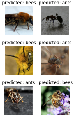
■ 위와 같은 방법들로 미리 학습된 가중치 파라미터가 포함된 사전 학습된 모델을 불러온 다음, 사전 학습된 모델의 완전연결 계층 이전의 가중치가 학습되지 않도록 설정해야 한다. 이를 가중치를 동결한다고 표현하며, 새로운 FC 계층만 학습을 진행해서 가중치를 업데이트한다. 이 과정을 fine-tuning이라 한다.
■ 예를 들어 model2와 같은 구조에 fine-tuning을 진행하려면, model2는 맨 상위 층 하나만 FC 층이므로 해당 층을 제외한 신경망의 모든 층의 requires_grad를 False로 설정해서 파라미터를 동결하면 된다.
model_conv = models.resnet18(weights='IMAGENET1K_V1')
for param in model_conv.parameters():
    param.requires_grad = False

# 새로 생성된 모듈의 매개변수는 기본값이 requires_grad=True 임
num_ftrs = model_conv.fc.in_features
model_conv.fc = nn.Linear(num_ftrs, 2) # num_ftrs = 512
- 이렇게 하면 model2 구조와 동일한 구조인 model_conv는 FC 층만 동결이 해제된 상태가 된다.
model_conv = model_conv.cuda()
optimizer_conv = optim.SGD(model_conv.fc.parameters(), lr=0.001, momentum=0.9)
scheduler_conv = optim.lr_scheduler.StepLR(optimizer_conv, step_size=10, gamma=0.1)
criterion = nn.CrossEntropyLoss().cuda()
model_conv = train_model(model_conv, criterion, optimizer_conv, scheduler_conv, num_epochs=20)
```#결과#```
Epoch 0/19
----------
train Loss: 0.4327 Acc: 0.7951
val Loss: 0.2201 Acc: 0.9020

Epoch 1/19
----------
train Loss: 0.5052 Acc: 0.7787
val Loss: 0.2073 Acc: 0.9412

Epoch 2/19
----------
train Loss: 0.3750 Acc: 0.8279
val Loss: 0.2069 Acc: 0.9346

...,
...,
Epoch 18/19
----------
train Loss: 0.3170 Acc: 0.8811
val Loss: 0.2149 Acc: 0.9412

Epoch 19/19
----------
train Loss: 0.4102 Acc: 0.8320
val Loss: 0.1832 Acc: 0.9542
````````````
visualize_model(model_conv)
plt.ioff()
plt.show()
■ 학습을 진행하면 진행 속도가 더 빨라지는 것을 확인할 수 있는데, 이는 신경망에서 FC 층을 제외한 모든 계층이 동결되어 있으므로 FC 층을 제외한 다른 층에서의 그래디언트를 계산할 필요가 없기 때문이다.
■ 전이 학습은 이렇게 데이터가 적을 때 사전 학습된 모델을 파인튜닝하는 기법으로, 사전 학습된 모델에 수많은 이미지 데이터를 학습시켜 놓았기 때문에 이 이미지들의 feature를 활용하는 것이다.
■ 예를 들어 사전 학습된 모델은 수백만 장의 개, 고양이, 사람, 곤충 등 다양한 종류의 이미지의 feature를 학습시켰을 것이다. 그렇기 때문에 사용자가 분류하고자 하는 이미지의 feature들도 학습시켰을 가능성이 높다.
'파이토치' 카테고리의 다른 글
| 파이토치 합성곱 신경망(CNN) (1) (0) | 2024.12.05 |
|---|---|
| torch.nn (2) (0) | 2024.12.04 |
| torch.nn (1) (0) | 2024.12.04 |

